Phaedra: Learning High-Fidelity Discrete Tokenization for the Physical Sciences

Lingsch, Levi; Kissas, Georgios; Jakubik, Johannes; Mishra, Siddhartha

Phaedra: Learning High-Fidelity Discrete Tokenization for the Physical Sciences

Levi Lingsch^1,2,3, Georgios Kissas⁴, Johannes Jakubik², Siddhartha Mishra^1,3

¹ETH AI Center, ²IBM Research Europe, ³ SAM ETH Zurich, ⁴SDSC

NeurIPS 2026

Paper Code arXiv 🤗 Models 🤗 Tokenized data

Disentangled Latent Control: Phaedra factorizes fields into independent $z_\mu$ (Morphology) and $z_\alpha$ (Amplitude) tokens. By combining, for example, the local vortices from Sample B ($z_{\mu,B}$) with the global magnitude profile of Sample A ($z_{\alpha,A}$), the reconstruction maintains the fine-scale turbulent structure of one while strictly obeying the physical dynamic range of the other.

Abstract

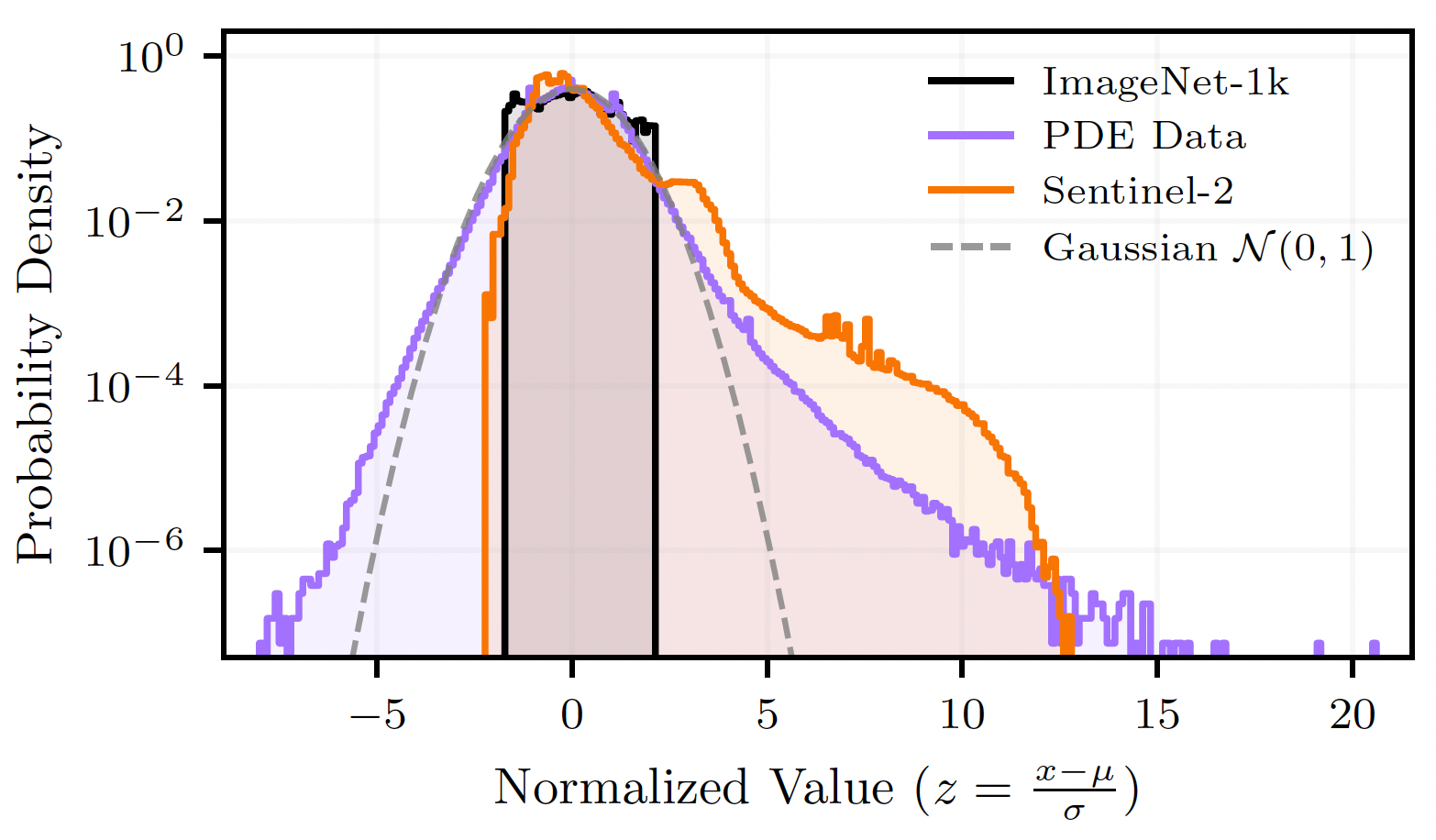
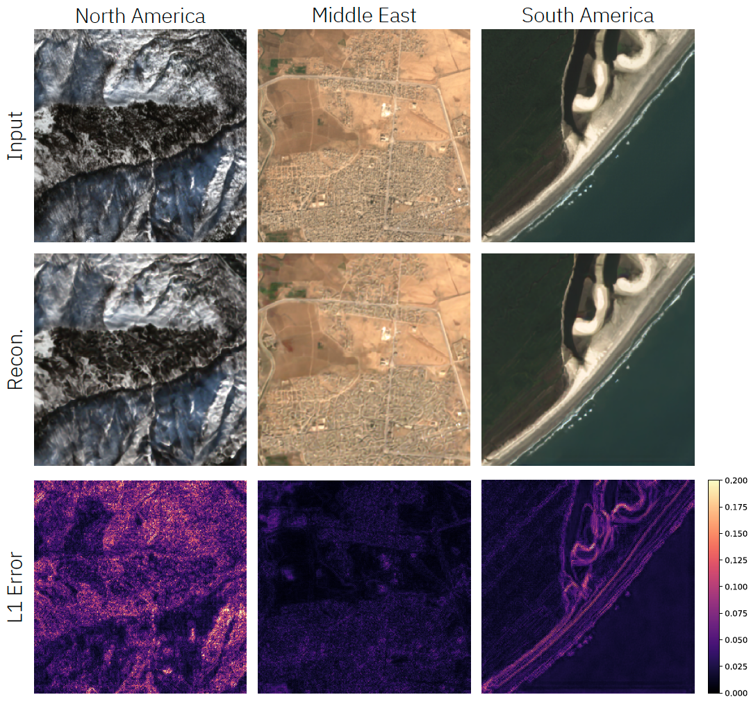
Tokens are discrete representations that allow modern deep learning to scale by transforming high-dimensional data into sequences that can be efficiently learned. As existing tokenizers are designed for realistic visual perception, we investigate whether these are optimal for scientific images, which exhibit a large dynamic range and require token embeddings to retain physical properties. We propose Phaedra, inspired by classical shape-gain quantization and proper orthogonal decomposition. We demonstrate that Phaedra consistently improves reconstruction across a range of PDE datasets and shows strong out-of-distribution generalization to unknown PDEs and real-world Earth observation data.

Phaedra consistently improves reconstruction across PDE datasets, capturing fine details and precise magnitudes critical for scientific simulation. This is achieved by splitting the embeddings into shape and gain components, allowing for high-fidelity tokenization that retains physical properties, even in out-of-distribution scenarios.

Data distributions after normalization. Natural images have a fixed range and uniform distribution, even after normalization. Physical datasets, however, have a much larger range of values with outliers far outside the nominal range.

Methodology

Phaedra leverages a disentangled hierarchical representation inspired by shape-gain quantization. The tokenizer factorizes latent embeddings into two distinct components: morphology ($z_\mu$), which captures spatial structures and topological features via Finite Scalar Quantization (FSQ), and amplitude ($z_\alpha$), which preserves the dynamic range and physical magnitudes. By incorporating an approximately continuous channel for amplitude, Phaedra avoids the precision loss common in standard discrete codebooks. This architecture effectively mirrors Proper Orthogonal Decomposition (POD) by separating spatial modes from their scalar coefficients, ensuring that physical properties such as conservation laws and sharp gradients are maintained even at high compression ratios.

The Phaedra pipeline uses a single encoder to compute two sets of embeddings; the shape embeddings are quantized using sparse, high-dimensional FSQ to capture spatial structures, while the gain embeddings are passed through a dense, 1-dimensional quantizer which approximates a continuous channel, preserving physical magnitudes. Following quantization, a learned recombination operator combines these two embeddings and passes them to the decoder for the final reconstruction.

Interactive Latent Space Exploration

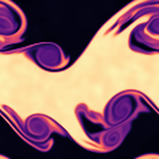
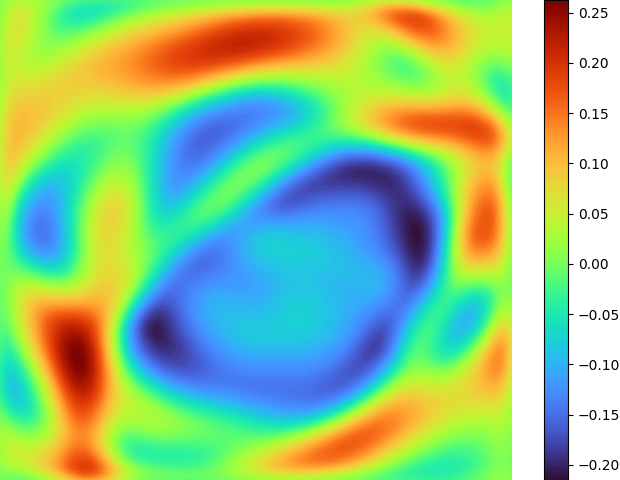
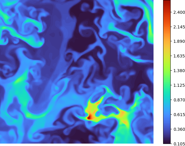
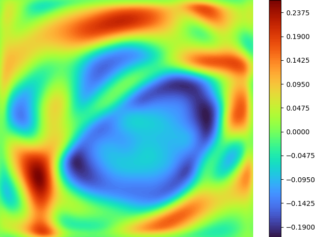
Use the sliders below to independently interpolate the morphology ($z_\mu$) and amplitude ($z_\alpha$) tokens between two timesteps of the Kelvin-Helmholtz (KH) instability dataset. This example illustrates the disentanglement of features via the amplitude-morphology latent representations. Interpolating between the amplitude tokens shows larger changes within the overall structure of the flow, while changing morphology tokens results in finer changes to the turbulent structures, while maintaining the same overall dynamic range. By combining the morphology of one sample with the amplitude of another, we can generate reconstructions that maintain the fine-scale turbulent structure of one sample while strictly obeying the physical dynamic range of the other. Please note, this example is only for illustrative purposes and does not represent a true interpolation in the latent space, as the model was not trained with an explicit disentanglement loss.

Morphology ($z_\mu$): 0.0

KH t=0.95 (A) KH t=1.00 (B)

Amplitude ($z_\alpha$): 0.0

KH t=0.95 (A) KH t=1.00 (B)

Active Reconstruction

PDE Reconstruction Benchmarks

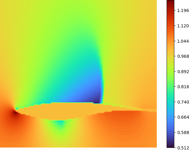
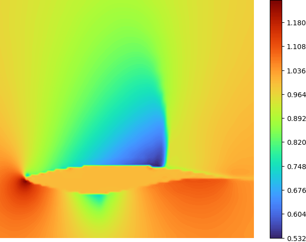
All models are trained on the same set of data, comprising Compressible Euler time-series defined by 4 different classes of initial conditions and Incompressible Navier-Stokes defined by 2 different classes of initial conditions. While we present some competitive tokenizers below, a comprehensive comparison against additional baselines is detailed in the main paper. We evaluate Phaedra across three levels of difficulty.

ID (In-Distribution): Test samples from the same PDE family and parameters as training.
OD₁ (Out-of-Distribution): Shifts in the PDE coefficients and initial conditions.
OD₂ (Out-of-Distribution): Shifts in the PDEs that define the problem.

ID: CEU Curved Riemann

OD₁: Airfoil

OD₂: Acoustic Wave

Model	Dataset	nMAE ↓	nRMSE ↓	Δσ²_loc ↓	γ_min ↑
VQ-VAE-2	ID	3.024	5.069	15.02	79.1%
	OD₁	2.113	5.854	21.55	87.5%
	OD₂	4.449	5.833	17.06	68.9%
FSQ	ID	2.603	4.292	11.29	85.3%
	OD₁	1.876	4.314	20.55	93.8%
	OD₂	3.831	4.997	11.65	68.0%
Phaedra (Ours)	ID	1.522	2.489	5.96	93.6%
	OD₁	1.217	2.442	6.47	98.0%
	OD₂	2.500	3.363	5.82	79.9%

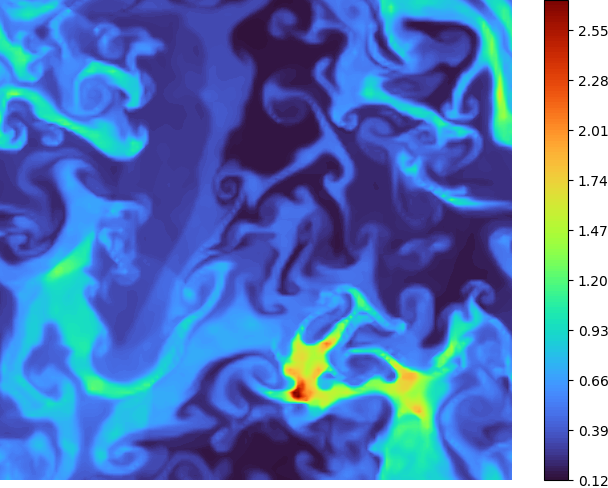
Sentinel-2 L1C Earth Observation Data

Zero-Shot Evaluation: All models were evaluated without fine-tuning on Earth Observation data, relying on representations learned from synthetic physical simulations.

Group	Model	rL₁ ↓	rL₂ ↓	Δσ²_loc ↓	γ_min ↑
Baseline	Continuous	7.426	8.100	62.61	90.02%
Compression: 4$\times$4	Phaedra₄ (Ours)	8.895	9.749	128.5	93.17%
Compression: 4$\times$4	FSQ₄	11.053	12.405	215.8	77.62%
Compression: 8$\times$8	Phaedra₈ (Ours)	9.900	11.475	163.9	62.72%
Compression: 8$\times$8	Cosmos₈	16.717	19.245	19,566	79.70%

Metrics calculated on native 13-band resolutions (10m, 20m, 60m).

Sentinel-2 Reconstruction results — Figure 1: Comparison of Ground Truth vs. Phaedra Reconstruction for Sentinel-2 L1C imagery.

Neural Operators on Phaedra Tokens

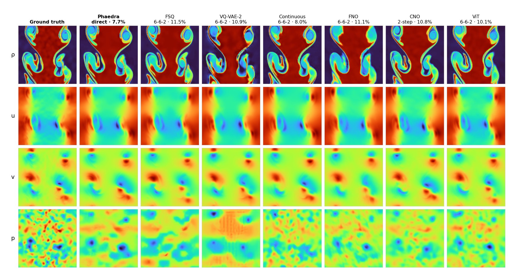
Tokens are only useful if models can learn on them. We train a 38M-parameter encoder–decoder transformer that maps the tokens of an initial condition, together with a lead time $t$, to the tokens at time $t$; the frozen Phaedra decoder turns the predicted tokens back into density, velocity and pressure. The same transformer is trained on FSQ and VQ-VAE-2 tokens and on the latents of a continuous autoencoder, and we compare with FNO, CNO and a ViT that work directly on the fields — every model has about 38M parameters (44M for the larger VQ-VAE-2 vocabularies) and is trained separately on three compressible Euler datasets from Poseidon: Kelvin–Helmholtz (KH), curved Riemann (RC) and Riemann–Kelvin–Helmholtz (RKH), which the tokenizer never saw during its training.

Predicted tokens and the physics decoded from them

Variable:

The first test trajectory of each dataset, from $t = 0$ to the final time $t = 0.7$. From left to right: the ground truth; the amplitude and morphology tokens predicted by the transformer on the 32×32 token grid (morphology tokens are coloured by their FSQ code); the field decoded from these tokens; and the absolute error, labelled with the relative $L_1$ error of the frame. Every frame is predicted in a single step from the tokens of the initial condition; the first frame shows the tokenized initial condition and its reconstruction. The video is rendered from the released weights (scripts/website/render_token_video.py), and its errors are identical to those in the evaluation below.

Accuracy at the final time

Relative $L_1$ error (%) at $t = 0.7$, averaged over $\rho, u, v, p$ and the 240 test trajectories of each dataset, ± the 95% bootstrap confidence interval. Every model is shown with its best prediction strategy (tag: d direct $0 \to t$, 2s autoregressive 2-step, 662 rollout $0 \to 0.3 \to 0.6 \to 0.7$); bold marks the best model per dataset. Phaedra tokens are the best of the discrete representations on all three datasets, with 16%, 28% and 43% lower error than FSQ tokens on KH, RC and RKH. They give the lowest error of all models on RC and RKH; on KH the ViT (9.18%) and the continuous-latent transformer (9.28%) are slightly more accurate than Phaedra (9.50%).

Model	Input	KH	RC	RKH
Phaedra transformer	Phaedra tokens	9.50 ± 0.34 d	27.21 ± 0.71 662	10.23 ± 0.80 662
FSQ transformer	FSQ tokens	11.28 ± 0.34 662	38.05 ± 1.05 662	17.99 ± 1.37 662
VQ-VAE-2 transformer	VQ-VAE-2 tokens	15.14 ± 0.48 662	42.40 ± 0.63 d	24.52 ± 1.15 662
Continuous transformer	continuous AE latents	9.28 ± 0.30 662	119.05 ± 2.96 d	11.56 ± 0.70 662
FNO	physical fields	12.55 ± 0.36 662	35.63 ± 0.69 662	16.66 ± 0.91 662
CNO	physical fields	10.15 ± 0.32 2s	29.92 ± 0.74 2s	11.82 ± 0.82 662
ViT	physical fields	9.18 ± 0.27 662	39.68 ± 0.58 d	13.20 ± 0.79 662

Per-variable errors ($\rho, u, v, p$) of all 21 models

Model	Data	ρ	u	v	p	Average	Strategy
Phaedra	KH	4.78	8.43	24.29	0.51	9.50 ± 0.34	direct
Phaedra	RC	20.66	40.73	40.42	7.02	27.21 ± 0.71	6-6-2
Phaedra	RKH	6.52	16.01	15.64	2.74	10.23 ± 0.80	6-6-2
FSQ	KH	5.30	10.91	28.27	0.62	11.28 ± 0.34	6-6-2
FSQ	RC	28.12	57.08	56.77	10.21	38.05 ± 1.05	6-6-2
FSQ	RKH	10.37	27.73	28.78	5.08	17.99 ± 1.37	6-6-2
VQ-VAE-2	KH	7.95	13.90	38.04	0.68	15.14 ± 0.48	6-6-2
VQ-VAE-2	RC	29.54	63.17	64.39	12.48	42.40 ± 0.63	direct
VQ-VAE-2	RKH	14.73	38.09	37.29	7.97	24.52 ± 1.15	6-6-2
Continuous	KH	4.64	8.34	23.53	0.61	9.28 ± 0.30	6-6-2
Continuous	RC	77.95	197.31	156.93	44.00	119.05 ± 2.96	direct
Continuous	RKH	7.09	18.09	17.87	3.18	11.56 ± 0.70	6-6-2
FNO	KH	6.24	11.18	32.23	0.54	12.55 ± 0.36	6-6-2
FNO	RC	26.31	53.62	53.42	9.16	35.63 ± 0.69	6-6-2
FNO	RKH	10.08	26.36	25.67	4.54	16.66 ± 0.91	6-6-2
CNO	KH	5.06	9.10	25.93	0.51	10.15 ± 0.32	2-step
CNO	RC	22.65	44.44	44.66	7.94	29.92 ± 0.74	2-step
CNO	RKH	6.79	18.83	18.50	3.17	11.82 ± 0.82	6-6-2
ViT	KH	4.64	8.25	23.33	0.51	9.18 ± 0.27	6-6-2
ViT	RC	28.76	60.17	59.51	10.28	39.68 ± 0.58	direct
ViT	RKH	9.09	20.86	19.66	3.18	13.20 ± 0.79	6-6-2

All tables as CSV, Markdown and LaTeX: docs/results. The released RKH operators are the checkpoints evaluated in the paper: step 56k of the Phaedra transformer and epoch 59 of the continuous-latent transformer, whose training diverged afterwards.

Error over time

Relative $L_1$ error over the prediction horizon (mean over $\rho, u, v, p$ and the 240 test trajectories). The snapshots are $\Delta t = 0.05$ apart. Direct predicts every time in a single step from $t = 0$, 2-step chains predictions two snapshots ahead ($2\Delta t = 0.1$ per step, $0 \to 0.1 \to \dots \to 0.7$), and 6-6-2 rolls out $0 \to 0.3 \to 0.6 \to 0.7$. Click a model in the legend to hide it.

Dataset:

Strategy:

log scale

Ground truth and every operator at t = 0.7 (KH, first test trajectory) — The first test trajectory at the final time, all four variables. Each model is shown with the strategy of the table above; the label gives its average relative $L_1$ error on this trajectory. The colour scales follow the ground truth.

The tokenizer sets the floor

Decoding the ground-truth tokens of the test data gives the lowest error that any operator on a representation can reach. Phaedra's floor is 1.6–1.9× lower than that of FSQ and 2.3–2.5× lower than that of VQ-VAE-2 on the same 32×32 token grid; only the continuous autoencoder, which is not discrete, is lower. Relative $L_1$ error (%) at $t = 0.7$, mean over $\rho, u, v, p$.

Tokenizer	KH	RC	RKH
Phaedra	0.54	3.30	1.49
FSQ	1.01	5.16	2.36
VQ-VAE-2	1.37	8.39	3.45
Continuous AE (not discrete)	0.27	1.48	0.65

Masked Autoencoding on Token Grids

Phaedra tokens also support self-supervised learning. A masked autoencoder (a transformer with about 48M parameters) sees a token grid with 75% of its tokens hidden and reconstructs them. It is pre-trained on KH, RC and RKH together and then fine-tuned on each dataset. The table gives the relative $L_1$ error (%) of the fields decoded from the reconstructed token grids, mean over $\rho, u, v, p$ (number of test trajectories in parentheses).

Tokens	pre-trained on 3 PDEs evaluated on RKH	fine-tuned evaluated on KH	fine-tuned evaluated on RC	fine-tuned evaluated on RKH
Phaedra	16.43 (10 traj.)	4.76 (10 traj.)	22.17 (10 traj.)	7.27 (10 traj.)
FSQ	16.91 (10 traj.)	6.29 (1 traj.)	28.20 (1 traj.)	7.07 (1 traj.)

The masks are random, so each number comes from one evaluation run. The fine-tuned FSQ models were evaluated on a single test trajectory.

Code, Models and Data

Code

The tokenizer (also as a small pip-installable package), token generation, the 21 neural operators, masked autoencoding, and the evaluation that reproduces every number on this page. MIT license.

🤗 Models

Four tokenizers (Phaedra, FSQ, VQ-VAE-2, continuous AE), the 21 neural operators and eight masked autoencoders as safetensors, each with its training configuration. CC BY-NC 4.0.

🤗 Tokenized data

Phaedra, FSQ and VQ-VAE-2 tokens and continuous latents of KH, RC and RKH: 10,000 trajectories with 21 time steps each (44 GB). CC BY-NC 4.0, following the Poseidon source data.

Tokenize a field

git clone https://github.com/camlab-ethz/Phaedra.git && cd Phaedra && pip install -e .

import torch
from phaedra import load_pretrained

model = load_pretrained()                        # the paper's tokenizer, downloaded from Hugging Face
x = torch.randn(1, 1, 128, 128)                  # a field normalized per variable: (x - mean) / std
quant, _, (morph, amp), _ = model.encode(x)      # morphology and amplitude tokens on the 32x32 grid
x_rec = model.decode(quant)

Reproducing the operator and MAE results, training from scratch and preparing the Poseidon data are described in the README.

Conclusion & Discussion

Our findings demonstrate that Phaedra successfully closes the "fidelity gap" that typically limits discrete tokenization in scientific applications. By balancing structural discretization with magnitude preservation, the model achieves superior reconstruction across diverse PDE families and exhibits remarkable zero-shot transfer to complex Earth observation data. The higher fidelity carries over to learning on the tokens: neural operators trained on Phaedra tokens are more accurate than those trained on the other discrete tokenizers. This suggests that the shape-gain prior serves as a fundamental inductive bias for physical systems, enabling models to generalize across scales and disciplines. As we move toward larger scientific foundation models, Phaedra provides a robust framework for transforming continuous physical fields into discrete sequences without sacrificing the precision required for rigorous scientific analysis.

BibTeX

@inproceedings{lingsch2026phaedra,
  title         = {Phaedra: Learning High-Fidelity Discrete Tokenization for the Physical Sciences},
  author        = {Lingsch, Levi and Kissas, Georgios and Jakubik, Johannes and Mishra, Siddhartha},
  booktitle     = {Advances in Neural Information Processing Systems},
  year          = {2026},
  eprint        = {2602.03915},
  archivePrefix = {arXiv},
  url           = {https://arxiv.org/abs/2602.03915}
}